Understanding RNNs

Recurrent Neural Networks

Linear layers and convolutional layers are very popular in neural network architectures. So what is the need of Recurrent Neural Networks? There is an obvious limitation to the former architectures. Can you guess what it is?
.
.
.
.
Memory!
These architectures don’t store any information about the previous inputs given to the network. This mean they tend to give poor results while working with sequential data (for the most part). Humans don’t start thinking from scratch at every instant. Just while reading this sentence, you have an idea of the words which came before and the ones to follow. A linear model processes each input independently. So you must convert the entire sequence into one input data point. Hence, they are stateless.

What is an RNN?

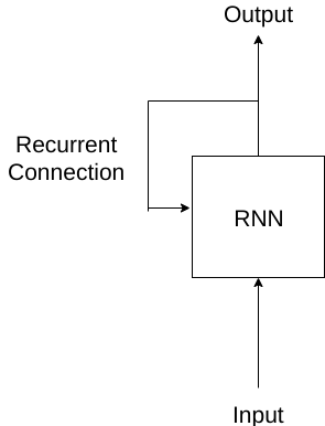
An RNN is an architecture which unlike Linear models, preserve state. They process sequences by iterating through its elements and maintaining a state. This state is reset while processing two different sequences. This is what a simple RNN looks like:

The saved state is called the hidden state. An RNN processes each element of the sequence sequentially. At each time step, it updates its hidden state and produces an output. This is what happens when we unroll an RNN:

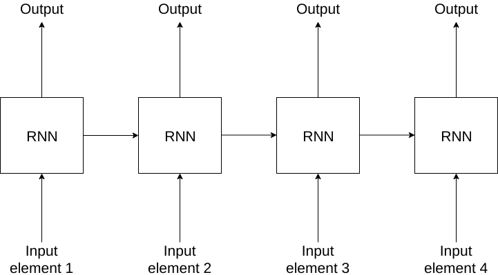
Unrolling an RNN is simply visualizing how it processes the sequence element by element. In reality, the RNN consists of just one cell processing the input in a loop. This property of an RNN allows it to process variable length inputs. RNNs are just a refactored, fully-connected neural network.

The working of an RNN (at timestep \(t\)) is as follows: An RNN consists of 3 weight matrices: \(W_x\), \(W_h\), \(W_y\).

• \(W_x\) is the weight matrix for the input (x).
• \(W_h\) is the weight matrix for the hidden state.
• \(W_y\) is the weight matrix for the output.

The hidden state is given by:
\(H_t = \sigma(W_x * X_t + W_h * H_{t-1})\)

• \(H_t\) is the hidden state at timestep \(t\).
• \(\sigma\) is the activation function (generally sigmoid or tanh).
• \(X_t\) is the input at the current timestep.

The output of the RNN is given by:
\(y = \sigma_y(W_y * H_t)\)

Due to the sequential nature of natural language, RNNs are commonly used in Natural Language Processing. Let us try to better understand the working of RNNs using an example.

In this example we are going to build a model to classify names into two countries of origin -> Italy and Germany. Our dataset consists of two files Italian.txt and German.txt. Both of these files contain a single name on each line. The data can be downloaded by:

1
wget https://download.pytorch.org/tutorial/data.zip

After unzipping the downloaded file, you will find several files which follow the following format:

name_1
name_2
name_3
...

Cleaning the Data

We start off by importing all the modules we will be using for this project. The only module you will need to install is of course pytorch.

1
2
3
4
5
6
7
import torch
from torch import nn
from torch.nn import functional as F
from torch.utils.data import Dataset, DataLoader, random_split
from pprint import pprint
import os
from string import ascii_letters

Reading the data

1
2
3
4
5
6
7
with open('Projects/NameClassifier/data/names/German.txt', 'r') as german_f, open('Projects/NameClassifier/data/names/Italian.txt', 'r') as italian_f:
    german_names = german_f.read()
    italian_names = italian_f.read()

print(f'German names:\n{german_names[:30]}')
print()
print(f'Italian names:\n{italian_names[:33]}')

Output:

German names:
Abbing
Abel
Abeln
Abt
Achilles

Italian names:
Abandonato
Abatangelo
Abatantuono

Finding all the unique characters in the files

The classifier which we are going to build is going to be character based. This means that it will take a sequence of characters as its input. Each name will be read by the model character by character. For this we need to first find all the unique characters in the files. We find all the unique characters in the files and then take its union with all letters (uppercase and lowercase) to form our vocabulary.

1
2
3
unique_characters = set((german_names + italian_names).replace('\n', '')).union(set(ascii_letters))
unique_characters = list(unique_characters)
''.join(sorted(unique_characters))

Output:

" 'ABCDEFGHIJKLMNOPQRSTUVWXYZabcdefghijklmnopqrstuvwxyzßàäèéìòóöùü"

Doing this ensures that our vocabulary will contain as many used characters as possible. You can probably get away with just using ascii_letters to form your vocabulary. This is what our list of names looks like:

1
2
3
4
german_names = german_names.split('\n')
italian_names = italian_names.split('\n')
print(german_names[:5])
print(italian_names[:5])

Output:

['Abbing', 'Abel', 'Abeln', 'Abt', 'Achilles']
['Abandonato', 'Abatangelo', 'Abatantuono', 'Abate', 'Abategiovanni']

Removing common names

We don’t want our classifier to accept the same input with two different classes. Hence, we will find the names which exist in both the german and italian datasets and remove them from both

1
2
common_names = list(set(german_names).intersection(set(italian_names)))
common_names

Output:

['', 'Salomon', 'Paternoster']

After removing the common names:

1
2
3
4
5
6
for common_name in common_names:
    german_names.remove(common_name)
    italian_names.remove(common_name)
    
common_names = list(set(german_names).intersection(set(italian_names)))
common_names

Output:

[]

Creating our data

We will create a list of all our names. This will be the input passed to our model. Along with this we will also need labels. We will have a label of 0 for german names and a label of 1 for italian names.

1
2
3
4
5
6
7
german_label = [0]
italian_label = [1]

all_names = german_names + italian_names
all_labels = german_label * len(german_names) + italian_label * len(italian_names)
print(all_names[720:726])
print(all_labels[720:726])

Output:

['Zimmerman', 'Zimmermann', 'Abandonato', 'Abatangelo', 'Abatantuono', 'Abate']
[0, 0, 1, 1, 1, 1]

One hot encoding characters

For our model to be able to process our input, we have to convert the characters to one hot encoded vectors. The size of our vector will be the total number of unique characters in our dataset. Hence we will first create a mapping of our character and its index. We can then use this mapping to convert our input characters to digits.

1
2
stoi =  {char:idx for idx, char in enumerate(sorted(unique_characters))}
stoi

Output:

{' ': 0,"'": 1,'A': 2,'B': 3,'C': 4,'D': 5,'E': 6,'F': 7,'G': 8,'H': 9,'I': 10,'J': 11,'K': 12,'L': 13,'M': 14,'N': 15,'O': 16,'P': 17,'Q': 18,'R': 19,'S': 20,'T': 21,'U': 22,'V': 23,'W': 24,'X': 25,'Y': 26,'Z': 27,'a': 28,'b': 29,'c': 30,'d': 31,'e': 32,'f': 33,'g': 34,'h': 35,'i': 36,'j': 37,'k': 38,'l': 39,'m': 40,'n': 41,'o': 42,'p': 43,'q': 44,'r': 45,'s': 46,'t': 47,'u': 48,'v': 49,'w': 50,'x': 51,'y': 52,'z': 53,'ß': 54,'à': 55,'ä': 56,'è': 57,'é': 58,'ì': 59,'ò': 60,'ó': 61,'ö': 62,'ù': 63,'ü': 64}

While our RNN can accept inputs of variable length, we still have to define a sequence length. This will allow us to batch our data for parallel execution.

1
2
3
4
5
6
7
8
9
10
11
12
13
14
15
16
17
18
19
20
21
def one_hot_encoder(name, sequence_length):
    global stoi
    size = len(stoi)
    print(f'Size of stoi: {size}')
    # To save output
    encoded = []
    # Iterating through name
    for char in name:
        temp = torch.zeros(size)
        # Setting index of character to 1
        temp[stoi[char]] = 1
        encoded.append(temp)
        
    # Filling the rest of the sequence with zeros
    for i in range(sequence_length - len(name)):
        temp = torch.zeros(size)
        encoded.append(temp)

    return torch.stack(encoded)

one_hot_encoder('Aniket', 10)

Size of stoi: 65
tensor([[0., 0., 1., 0., 0., 0., 0., 0., 0., 0., 0., 0., 0., 0., 0., 0., 0., 0.,
            0., 0., 0., 0., 0., 0., 0., 0., 0., 0., 0., 0., 0., 0., 0., 0., 0., 0.,
            0., 0., 0., 0., 0., 0., 0., 0., 0., 0., 0., 0., 0., 0., 0., 0., 0., 0.,
            0., 0., 0., 0., 0., 0., 0., 0., 0., 0., 0.],
        [0., 0., 0., 0., 0., 0., 0., 0., 0., 0., 0., 0., 0., 0., 0., 0., 0., 0.,
            0., 0., 0., 0., 0., 0., 0., 0., 0., 0., 0., 0., 0., 0., 0., 0., 0., 0.,
            0., 0., 0., 0., 0., 1., 0., 0., 0., 0., 0., 0., 0., 0., 0., 0., 0., 0.,
            0., 0., 0., 0., 0., 0., 0., 0., 0., 0., 0.],
       ...

Creating our dataset object

Now we have done a lot of preprocessing! Let us combine all of this in our dataset class. We will set the sequence length to \(18\) as that is the length of the longest name in our dataset.

1
2
3
4
5
6
7
8
9
10
11
12
13
14
15
16
17
18
19
20
21
22
23
24
25
26
27
28
29
30
31
32
33
34
35
36
37
38
39
40
41
42
43
44
45
46
47
48
49
50
51
52
53
54
55
56
57
58
59
60
61
class NameDataset(Dataset):
    def __init__(self, german_fname='Projects/NameClassifier/data/names/German.txt', italian_fname='Projects/NameClassifier/data/names/Italian.txt'):
        super().__init__()
        # Reading from files
        with open(german_fname, 'r') as german_f, open(italian_fname, 'r') as italian_f:
            german_names = german_f.read()
            italian_names = italian_f.read()
        
        # Finding unique characters
        unique_characters = list(set((german_names + italian_names).replace('\n', '')).union(set(ascii_letters)))
        german_names = german_names.split('\n')
        italian_names = italian_names.split('\n')
        
        # Removing common names
        common_names = list(set(german_names).intersection(set(italian_names)))
        for common_name in common_names:
            german_names.remove(common_name)
            italian_names.remove(common_name)
        german_label = [0]
        italian_label = [1]

        # Setting names and labels
        self.names = german_names + italian_names
        self.labels = german_label * len(german_names) + italian_label * len(italian_names)
        
        # Mapping from chars to int
        self.stoi =  {char:idx for idx, char in enumerate(sorted(unique_characters))}
        
        # Size of longest word is 18
        self.sequence_length = 18
        
        # One hot encoded names
        self.encoded_names = self.encode_dataset()

    def one_hot_encoder(self, name):
        size = len(self.stoi)

        encoded = []
        for char in name:
            temp = torch.zeros(size)
            temp[self.stoi[char]] = 1
            encoded.append(temp)

        for i in range(self.sequence_length - len(name)):
            temp = torch.zeros(size)
            encoded.append(temp)

        return torch.stack(encoded)
        
    def encode_dataset(self):
        encoded_list = []
        for name in self.names:
            encoded_list.append(self.one_hot_encoder(name))
            
        return torch.stack(encoded_list)
        
    def __len__(self):
        return len(self.labels)
    
    def __getitem__(self, idx):
        return self.encoded_names[idx], torch.tensor([self.labels[idx]])

Let us see what our output looks like:

1
2
names = NameDataset()
names[0]

Output:

(tensor([[0., 0., 1.,  ..., 0., 0., 0.],
            [0., 0., 0.,  ..., 0., 0., 0.],
            [0., 0., 0.,  ..., 0., 0., 0.],
            ...,
            [0., 0., 0.,  ..., 0., 0., 0.],
            [0., 0., 0.,  ..., 0., 0., 0.],
            [0., 0., 0.,  ..., 0., 0., 0.]]), tensor([0]))

1
2
# Shape of input tensor (one word)
names[0][0].shape

Output:

torch.Size([18, 65])

1
2
3
4
5
6
7
8
device = 'cuda' if torch.cuda.is_available() else 'cpu'
split_ratio = 0.8
data_len = len(names)
train_size = int(split_ratio * data_len)
test_size = data_len - train_size

# Randomly splits data into given sizes
train_dataset, test_dataset = random_split(names, lengths=(train_size, test_size))

Comparison with a Linear model

Before we build our RNN based model, let us look at the results with a conventional Linear model. On our problem statement, using a model with just 3 linear layers, I was able to achieve an accuracy of just 69.2% even after training for 100 epochs. This problem is very simple with very short sequences. For a problem with longer sequences, the model’s performance would be even worse.

Building an RNN using linear layers

Let us revisit the mathematics behind an RNN: \(H_t = \sigma(W_x * X_t + W_h * H_{t-1})\) \(y = \sigma_y(W_y * H_t)\)

Where \(H_t\) is the hidden state at timestep \(t\) and \(y\) is the output of the RNN. For illustration purposes we will assume the batch size to be \(1\). Let us discuss some of the terminology commonly used while talking about RNNs.

Sequence length

Although RNNs can handle inputs of varying sequence lengths, tensor operations require the every sequence of the same size. This is why while RNNs can accept sequences of any length, for parallel processing we will maintain the same sequence length for every input batch. The sequence length for our model is \(18\) because that is the length of the longest name in our dataset.

Input size

This parameter of our RNN is different from the sequence length. This parameter signifies the size of one element of the sequence. For our example, the input size is \(65\) which is the size of our one hot encoded vector.

Now let us try building our own RNN with just linear layers. We will use nn.Linear for a linear layer. We need a linear layer for \(W_x, W_h\) and \(W_y\) each. We will also initialize the hidden state with torch.zeros. We will have a for loop to iterate through the sequence.

1
2
3
4
5
6
7
8
9
10
11
12
13
14
15
16
17
18
19
20
21
22
23
24
25
26
27
28
29
30
31
32
class LinearRNN(nn.Module):
    def __init__(self):
        super().__init__()
        global device
        self.device = device
        self.hidden_size = 256
        self.sequence_length = 18
        self.input_size = 65
        self.Wx = nn.Linear(self.input_size, self.hidden_size)
        self.Wh = nn.Linear(self.hidden_size, self.hidden_size)
        self.Wy = nn.Linear(self.sequence_length * self.hidden_size, self.hidden_size)
        self.h = torch.zeros(1, self.hidden_size).to(self.device)
        self.output_layer = nn.Linear(self.hidden_size, 2)
        
    def forward(self, input_tensor):
        h = torch.zeros(1, self.hidden_size).to(self.device)
        res = []
        # input_tensor.shape[1] = sequence length
        for i in range(input_tensor.shape[1]):     
            # input_tensor[:, i] = the ith element in the sequence
            x = F.tanh(self.Wx(input_tensor[:, i]))     
            h = F.tanh(self.Wh(h))
            h = torch.add(h, x)
            res.append(h)
        
        self.h = h.detach()        
        res = torch.stack(res, dim=1)
        res = res.reshape(-1, self.sequence_length * self.hidden_size)
        res = F.relu(self.Wy(res))
        res = self.output_layer(res)
        return res
    

Now let us create our DataLoader and set some hyperparameters before training the model.

1
2
3
4
5
6
7
8
9
10
11
12
13
14
15
batch_size = 1
linear_train_loader = DataLoader(train_dataset, batch_size=batch_size)
linear_test_loader = DataLoader(test_dataset, batch_size=batch_size)
model = LinearRNN().to(device)
criterion = nn.CrossEntropyLoss()
lr = 5e-6
optimizer = torch.optim.Adam(model.parameters(), lr=lr)
num_epochs = 30
max_accuracy = 0.0
MODEL_PATH = ''
if os.path.exists(MODEL_PATH):
    print('Existing model found!')
    load_weights(model, MODEL_PATH)
else:
    print('No existing model found.')

This is what our model looks like:

No existing model found.
LinearRNN(
    (Wx): Linear(in_features=65, out_features=256, bias=True)
    (Wh): Linear(in_features=256, out_features=256, bias=True)
    (Wy): Linear(in_features=4608, out_features=256, bias=True)
    (output_layer): Linear(in_features=256, out_features=2, bias=True)
)

Now it time to finally train the model.

1
2
3
4
5
6
7
8
9
10
11
12
13
14
15
16
17
18
19
20
21
22
23
24
25
26
27
28
29
30
31
32
33
34
35
36
37
for epoch in range(num_epochs):
    model.train()
    epoch_loss = 0
    total = 0
    correct = 0
    print(f'Epoch: {epoch}')
    for input_batch, labels in linear_train_loader:
        if labels.size(0) != batch_size: continue
        model.zero_grad()
        output = model.forward(input_batch.to(device))
        loss = criterion(output, labels.to(device).long().reshape(batch_size,))
        loss.backward()
        optimizer.step()
        epoch_loss += loss.item()
        total += labels.size(0)
        correct += torch.sum(torch.argmax(output, dim=1).view(1, -1) == labels.to(device).view(1, -1)).item()

    print(f'Accuracy: {correct/total * 100}\nLoss: {epoch_loss/total}')
    if (epoch + 1) % 3 == 0:
        test_epoch_loss = 0
        total = 0
        correct = 0
        model.eval()
        for input_batch, labels in linear_test_loader:
            with torch.no_grad():
                if labels.size(0) != batch_size: continue
                output = model.forward(input_batch.to(device))
                loss = criterion(output, labels.to(device).long().reshape(batch_size,))
                test_epoch_loss += loss.item()
                total += labels.size(0)
                correct += torch.sum(torch.argmax(output, dim=1).view(1, -1) == labels.to(device).view(1, -1)).item()

        test_accuracy = round(correct/total, 4) * 100
        print(f'''### TESTING ###
        Accuracy: {test_accuracy}
        Loss: {round(test_epoch_loss/total, 4)}''')

Output:

Epoch: 0
Accuracy: 61.85476815398076
Loss: 0.6853206089892516
Epoch: 1
Accuracy: 75.32808398950131
Loss: 0.6586288675235639
Epoch: 2
Accuracy: 82.76465441819772
Loss: 0.6005860694854382
### TESTING ###
        Accuracy: 82.87
        Loss: 0.5592
...
...
...
Epoch: 27
Accuracy: 95.18810148731409
Loss: 0.3622470853209808
Epoch: 28
Accuracy: 95.2755905511811
Loss: 0.3614634818813828
Epoch: 29
Accuracy: 95.53805774278216
Loss: 0.3607256871925981
### TESTING ###
        Accuracy: 92.31
        Loss: 0.394

As you can see, with just 30 epochs of training we are able to achieve testing accuracy of more than 92%! The RNN implementation we saw above is just to provide insight into the working of RNNs and I don’t recommend anyone to actually build their own RNNs while working on their projects. We will now use the torch.nn.RNN module on the same problem. This is a much faster implementation which supports parallel processing.

1
2
3
4
5
6
7
8
9
10
11
12
13
14
15
16
17
18
19
20
21
22
23
24
25
26
27
28
29
30
31
class NameClassifier(nn.Module):
    def __init__(self, max_len=18, hidden_size=256, input_size=65):
        super().__init__()
        dropout_prob = 0.4
        self.input_size = input_size
        self.sequence_length = max_len
        self.hidden_size = hidden_size
        self.num_layers = 2
        self.rnn = nn.RNN(
            input_size=self.input_size,
            hidden_size=self.hidden_size, 
            num_layers=self.num_layers, 
            batch_first=True,
            dropout=dropout_prob
        )
        self.dropout_layer = nn.Dropout(dropout_prob)
        self.linear_layer = nn.Linear(self.hidden_size * self.sequence_length, 256)
        self.output_layer = nn.Linear(256, 2)
        
        
    def forward(self, input_tensor, hidden):
        rnn_output, new_hidden = self.rnn(input_tensor, hidden)
        rnn_output = self.dropout_layer(rnn_output)
        linear_output = F.relu(self.linear_layer(rnn_output.reshape(-1, self.hidden_size * self.sequence_length)))
        output = F.softmax(self.output_layer(linear_output))
        new_hidden = new_hidden.detach()
        return output, new_hidden
        
        
    def init_hidden(self, batch_size):
        return torch.zeros(self.num_layers, batch_size, self.hidden_size)

The only difference between this model and the one which we built is the addition of nn.Dropout which helps the model to generalize better and prevents overfitting. For this particular problem this addition did not add much of a difference to the results but it is good practice to have some sort of regularization and it does not harm our results in any way. Setting hyperparameters and training:

1
2
3
4
5
6
model = NameClassifier().to(device)
criterion = nn.CrossEntropyLoss()
lr = 5e-6
optimizer = torch.optim.Adam(model.parameters(), lr=lr)
num_epochs = 30
max_accuracy = 0.0

This is what the nn.RNN model looks like.

Output:

NameClassifier(
    (rnn): RNN(65, 256, num_layers=2, batch_first=True, dropout=0.4)
    (dropout_layer): Dropout(p=0.4)
    (linear_layer): Linear(in_features=4608, out_features=256, bias=True)
    (output_layer): Linear(in_features=256, out_features=2, bias=True)
)

1
2
3
batch_size = 8
train_loader = DataLoader(train_dataset, batch_size=batch_size)
test_loader = DataLoader(test_dataset, batch_size=batch_size)

Training the model:

1
2
3
4
5
6
7
8
9
10
11
12
13
14
15
16
17
18
19
20
21
22
23
24
25
26
27
28
29
30
31
32
33
34
35
36
37
38
39
40
41
42
43
for epoch in range(num_epochs):
    model.train()
    epoch_loss = 0
    total = 0
    correct = 0
    hidden = model.init_hidden(batch_size=batch_size)
    print(f'Epoch: {epoch}')
    for input_batch, labels in train_loader:
        if labels.size(0) != batch_size: continue
        model.zero_grad()
        output, hidden = model.forward(input_batch.to(device), hidden.to(device))    
        loss = criterion(output, labels.to(device).long().reshape(batch_size,))
        loss.backward()
        optimizer.step()
        epoch_loss += loss.item()
        total += labels.size(0)
        correct += torch.sum(torch.argmax(output, dim=1).view(1, -1) == labels.to(device).view(1, -1)).item()
    
    print(f'Accuracy: {correct/total * 100}\nLoss: {epoch_loss/total}')
    if (epoch + 1) % 3 == 0:
        test_epoch_loss = 0
        total = 0
        correct = 0
        model.eval()
        hidden = model.init_hidden(batch_size=batch_size)
        for input_batch, labels in test_loader:
            with torch.no_grad():
                if labels.size(0) != batch_size: continue
                output, hidden = model.forward(input_batch.to(device), hidden.to(device))
                loss = criterion(output, labels.to(device).long().reshape(batch_size,))
                test_epoch_loss += loss.item()
                total += labels.size(0)
                correct += torch.sum(torch.argmax(output, dim=1).view(1, -1) == labels.to(device).view(1, -1)).item()

        test_accuracy = round(correct/total, 4) * 100
        print(f'''### TESTING ###
        Accuracy: {test_accuracy}
        Loss: {round(test_epoch_loss/total, 4)}''')
        if max_accuracy < test_accuracy:
            max_accuracy = test_accuracy
            save_weights(model, MODEL_PATH)
            print('Best model found!')
        

Output:

Epoch: 0
Accuracy: 51.58450704225353
Loss: 0.086549880848804
Epoch: 1
Accuracy: 51.6725352112676
Loss: 0.08647492449258415
Epoch: 2
Accuracy: 51.76056338028169
Loss: 0.08638013862598111
### TESTING ###
        Accuracy: 48.209999999999994
        Loss: 0.0864
Best model found!
...
...
...
Epoch: 27
Accuracy: 91.90140845070422
Loss: 0.049783599733466834
Epoch: 28
Accuracy: 92.6056338028169
Loss: 0.04917106074346623
Epoch: 29
Accuracy: 92.42957746478874
Loss: 0.04905853562161956
### TESTING ###
        Accuracy: 93.57
        Loss: 0.0475
Best model found!

As you can see we get very similar accuracies from the two models. This is because they are essentially doing the same thing.

Testing the model with user input

1
2
3
4
5
6
7
8
9
with torch.no_grad():
    model.eval()
    hidden = model.init_hidden(batch_size=1)
    input_tensor = names.one_hot_encoder('Tribbiani')
    input_tensor = input_tensor.view(1, *input_tensor.shape)
    output = model.forward(input_tensor.to(device), hidden.to(device))
    class_ = torch.argmax(output[0], dim=1).item()
    print('German' if class_ == 0 else 'Italian')
    print(f'Confidence: {output[0][0][class_]}')

Output:

Italian
Confidence: 0.9999949932098389

Drawbacks of the vanilla RNN

The RNN architecture which we have used until now (commonly called a “vanilla” RNN) is very simple and generally works for shorter sequence lengths. This is in part because of the vanishing gradient problem which affects vanilla RNNs. Due to this problem, the gradient signal from nearby hidden states (wrt time) is much larger when compared with that of farther hidden states. This leads to the model learning closer dependencies but failing to capture long term dependencies.
For example:
Q. The author of these books _______ coming to town.

• is
• are

The answer is of course ‘is’. This is because we are referring to the author and not to the books. This is called syntactic recency. The problem with RNNs is that they are able to identify sequential recency and might output ‘are’ as the blank follows the word ‘books’. Another reason as to why RNNs are unable to capture long term dependencies is that the hidden state is constantly being rewritten. This leads to continuous loss of information. Hence there is a need for better architectures which would be able to model short term as well as long term dependencies. There are two popularly used architectures namely:

1. Gated Recurrent Units (GRUs)
2. Long Short Term Memory (LSTMs)

GRUs

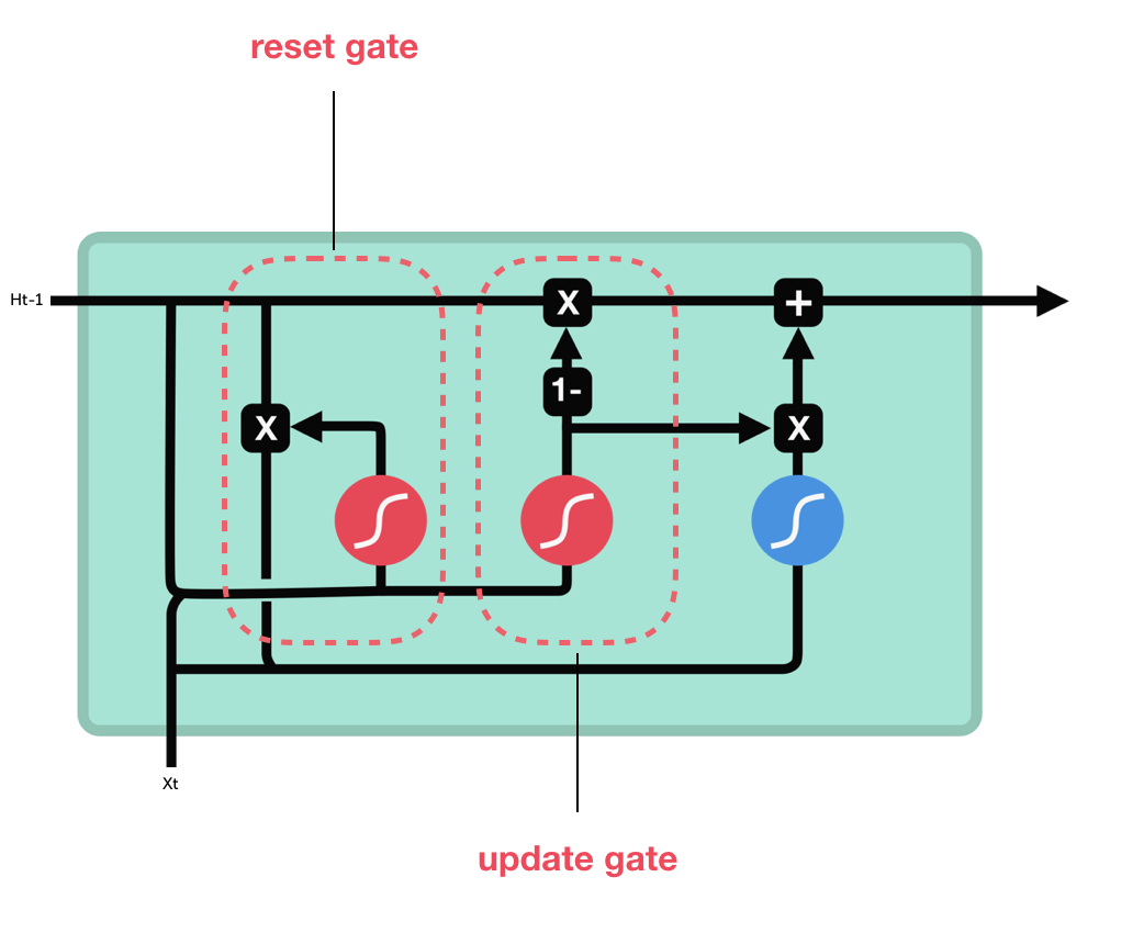
Here at each timestep \(t\), we have the input \(x^t\) and the hidden state \(h^t\). The GRU makes use of 2 gates:

1. The update gate:
   \(\large u^{(t)} = \sigma(W_u * h^{(t-1)} + U_u * x^{(t)} + b_u)\)
   Controls which parts of the hidden state are updated and which are preserved.

2. The reset gate:
   \(\large r^{(t)} = \sigma(W_r * h^{(t-1)} + U_r * x^{(t)} + b_r)\)
   Controls which parts of the previous hidden state are used to calculate new content.

These gates can be thought of as small Neural Networks which are used to calculate and extract relevant features and information from the input.

The reset gate is directly used to calculate the new hidden state content:
\(\large \tilde{h} = tanh\Big(W_h * (r^{(t)} \bullet h^{(t-1)}) + U_h * x^{(t)} +b_h\Big)\)

The new hidden state is calculated using the update gate. It simulatneously keeps what is kept from the previous hidden state and what is updated to the new hidden state.

How does a GRU solve the vanishing gradient problem?

GRUs make it easier to retain information long term. This can be done through the update gate. If the update gate is set to \(0\), the value of the new hidden state will become:
\(\large h^{(t)} = (1 - u^{(t)}) \bullet h^{(t-1)} + u^{(t)} \bullet \tilde{h}^{(t)}\)
But \(u^{(t)} = 0\)
Hence,
\(\large h^{(t)} = h^{(t-1)}\)

This means that the hidden state will never change. Hence from this example we can understand how the GRU will be able to capture long term or short term dependencies as it suites the problem.

LSTMs

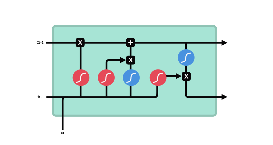
LSTMs are older and slightly more complex as compared to GRUs. They attempt to solve the vanishing gradient problem by having a separate memory called the cell state. This is separate from the hidden state. Theoretically this cell state can save information about the entire sequence. LSTMs use different gates to define how the cell state and hidden state are updated. Performance wise, there is no clear better alternative to use between GRUs and LSTMs. They have both outperformed each other at different tasks. GRUs due to their simpler structure are slightly faster to train and also easier to understand. Let us understand the working of the LSTM gates.

1. Forget gate
   In this gate the input and \(h_{t-1}\) is passed through a sigmoid function. This squishes the inputs between \(0\) and \(1\). The gate will “forget” values closer to \(0\) and “remember” values closer to \(1\).

2. Input gate
   This gate works in a similar fashion to the forget gate. It is used to extract relevant features from the input data. The output of this gate (from a sigmoid function) is again used to decide which parts of the input are important.

3. Output gate
   The output gate takes the cell state and the previous hidden state as input and calculates what the next hidden state should be.

4. Cell state
   The new cell state \(C_t\) is calculated using the outputs of the forget gate and the input gate.

Code

Using both LSTMs and GRUs in pytorch is very easy using nn.LSTM and nn.GRU. They follow a very similar API to that of nn.RNN and can provide better results for complex problems without much modification to the rest of the code.

Additional material

1. I have written another blog to build on your understanding using a project! Check out character based language model using RNNs.
2. Chris Olah’s post on RNNs and LSTMs.
3. Andrej Karpathy’s post on building an RNN from scratch.
4. A great lecture by Rachel Thomas as part of “A Code-First Introduction to Natural Language Processing”.